IMPORTANT NOTES:

• This assignment is to be carried out individually, and the assignment answers are to be submitted online on Moodle by each student;
• Each student must find their unique set of input values from the spread sheet on UNSW’s Moodle (CVEN3501 Assignment 2 individual values 2025.xlsx);
• For calculated (numerical) answers, round your values to 3 decimal digits;
• Please note that every set of dimensions and values is unique! There is no point in copying your mate’s results;
• Complete the student declaration form on Moodle. Until this is marked complete you will not be able to access the submission links;
• You will only have one try for entering your results in Moodle. Therefore, please make sure that you have done all your calculations and rechecked that they are correct before you enter your results;
• Penny for late submission is 5% per day.

Background

We often need to include the impact of groundwater pumping at a known rate in groundwater models. In this assignment you will build a simplified 2D numerical model to assess the impacts of pumping. The following differential equation describes 2D flow in a confined aquifer with a source or sink term R, here at a pumping node:

(1)    

Here, R > 0 for injection into the model, and R < 0 for abstraction from the model. Refer to your course notes for how to solve this equation using the finite difference approach in two dimensions. In all other nodes R = 0, so that pumping is only happening in one node.

You will need to consider how to modify Equation 1 to represent injection/abstraction from a uniform and isotropic aquifer using the finite difference method.

HINT: Consider the dimensions of the term R in Equation 1, they are not ^L / _T ³

The Problem

The objective of the assignment is to use Microsoft Excel to investigate the effect of changing boundary conditions on a rectangular isotropic and homogeneous confined aquifer, firstly without pumping and then including a groundwater pumping bore abstracting or injecting water. The assignment is based on the analysis by Frank and Reilly (1987).

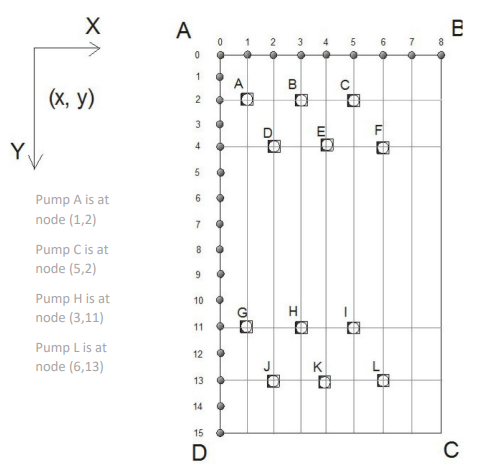
You should set up a model for your unique aquifer. Figure 1 is an example and does not necessarily match your aquifer dimensions. Your aquifer has an area X m wide (AB and CD) by Y m long (BC and DA). Use a finite difference discretization where Δx = Δy = 100 m. Your model will then be X’ nodes wide in the x-direction along boundaries AB and CD and Y’ nodes long in the y-direction along boundaries BC and DA.

In the example, the aquifer is X = 800 m wide by Y = 1500 m long and Δx = Δy = 100 m. This model therefore has X’ = 9 nodes in the x-direction (from node 0 to node 8 along boundaries AB and CD) and Y’ = 16 nodes in the y-direction (from node 0 to node 15 along boundaries BC and DA). See Figure 1.

Each student will have a unique set of data for the transmissivity (T [m²/day]), Pumping rate (Q [m³/day]), initial head conditions (h [m]), and an x-y coordinate representing the bore location. Find your data by searching your z-id in the excel sheet on Moodle (CVEN3501 Assignment 2 individual values 2025.xlsx). Figure 1 shows how the bore location x-y coordinates correspond to nodes in the numerical scheme.

For the spreadsheet to successfully iterate, circular references should be enabled. In Microsoft Excel 2010+ this is done under the menus: ”File” – ”Options” – ”Formulas”: Here you need to tick ”Enable iterative calculation”, set ”Maximum iterations” to 30,000 and ”Maximum change” to 0.0001.

Model the following two sets of aquifer conditions:

Model 1: The aquifer is surrounded by Dirichlet (fixed head) boundary conditions. Use a linear decrease in head from h m to 0 m along BC and AD, a fixed head of 0 m along boundary CD, and a fixed head of h m along boundary AB.

Model 2: The aquifer is surrounded by a mix of Dirichlet and Neumann (no flow) boundary conditions. Use a no-flow boundary condition (with ∂h/∂x = 0) across BC and AD, a fixed head of 0 m along boundary CD, and a fixed head of h m along boundary AB.

Provide the answers for the following questions in Moodle:

1. Calculate the flow though the aquifer for Model 1 without any abstraction. Hint: Check that the flow calculated by the spreadsheet is correct using Darcy’s Law [2 marks].
2. Calculate the flow though the aquifer for Model 2 without any abstraction. Hint: Check that the flow calculated by the spreadsheet is correct using Darcy’s Law [2 marks].
3. Using your unique values for the model dimensions, of the transmissivity, the bore node location and the abstraction or injection rate, calculate the water level (relative to the datum) at the given node location and the flows across each of the 4 boundaries for Model 1 (Dirichlet conditions). Note that abstraction (Q) is negative (by convention) for water leaving the aquifer. Calculate your flows over the boundaries as positive if into the aquifer and negative if out of the aquifer. Report the following: [10 marks]
   • a) Head at pumping node [m]
   • b) Flow through boundary AB [m³/d]
   • c) Flow through boundary DC [m³/d]
   • d) Flow through boundary AD [m³/d]
   • e) Flow through boundary BC [m³/d]
4. Again, using your unique values of the transmissivity, the bore node location and the pumping (or injection) rate given on the assignment sheet, calculate the water level (relative to the datum) at the given node location and the flows across each of the 4 boundaries for Model 2 (Dirichlet and Neumann conditions). Use the same convention for the direction of flow as in the preceding question. Report the following: [10 marks]
   • a) Head at pumping node [m]
   • b) Flow through boundary AB [m³/d]
   • c) Flow through boundary DC [m³/d]
   • d) Flow through boundary AD [m³/d]
   • e) Flow through boundary BC [m³/d]
5. For Model 2, what is the theoretically expected flow over boundary BC? [1 mark]

HINT: For Questions 3 and 4, please note that the transmissivity is given in [m²/day] and the abstraction/injection rate is in [m³/day].

Using your excel models, course notes, and the reference to Frank and Reilly (1987), answer the following multi-choice questions in Moodle [1 mark/question].

Please NOTE: the order (numeration) of the possible answers may be different in the Moodle submission link.

1. If the pumping rate doubles, what will happen to the drawdown at your pumping node (absolute magnitude of change)?
   • a) Drawdown doubles, for both models
   • b) Drawdown increases for model 1, and doubles for model 2
   • c) Drawdown doubles for model 1, and increases for model 2
   • d) Drawdown increases, for both models
   • e) No change in drawdown for either model
2. Based on your value for transmissivity, and assuming a uniform aquifer thickness of 5 m, this model most likely represents
   • a) An aquitard
   • b) A sand aquifer
   • c) A sandstone aquifer
   • d) A gravel aquifer
   • e) A fractured basalt aquifer
3. If you halve the discretisation of your model, i.e., from Δx = Δy = 100 m to Δx = Δy = 50 m, what will happen to the model truncation error?
   • a) Truncation error decreases by a factor of 2 (halves)
   • b) Truncation error decreases by more than a factor of 2
   • c) Truncation error increases by a factor of 2 (doubles)
   • d) Truncation error increases by less than a factor of 2
4. What best describes this model?
   • a) Anisotropic, homogenous, equilibrium, confined
   • b) Equilibrium, unconfined, heterogenous, isotropic
   • c) Homogenous, transient, isotropic, confined
   • d) Equilibrium, confined, homogenous, isotropic
   • e) Confined, transient, anisotropic, homogenous
5. Can the models be used to simulate temporal changes?
   • a) Yes, both
   • b) Yes, but only model 1
   • c) Yes, but only model 2
   • d) No, neither model
6. Can this model be used to model vertical flows?
   • a) Yes, both
   • b) Yes, but only model 1
   • c) Yes, but only model 2
   • d) No, neither model
7. Model boundary conditions are meant to represent the real boundaries of your groundwater system. Which of the following features would you model with a Dirichlet (fixed head) boundary?
   • a) The water table
   • b) A large lake
   • c) A non-conductive fault zone
   • d) A large granite outcrop
8. Model boundary conditions are meant to represent the real boundaries of your groundwater system. Which of the following features would you model with a Neumann (no flow) boundary?
   • a) A large lake
   • b) A large granite outcrop
   • c) A conductive fault zone
   • d) The water table
9. Based on your answers to all previous questions, which is the most important parameter for your models (i.e., what are your models most sensitive to)?
   • a) Pumping rate
   • b) Hydraulic conductivity
   • c) The choice of boundary conditions
   • d) The model software
   • e) The discretisation scheme
10. If you built an unconfined (water table) model, would the drawdown at your pumping well be smaller or larger (absolute magnitude of change)?
    • a) Smaller, for both models
    • b) Smaller for model 1, but larger for model 2
    • c) Larger for model 1, but smaller for model 2
    • d) Larger, for both models
    • e) The same, for both models

Reference:

Frank, C. L. and Reilly, T. E. (1987). The effects of boundary conditions on the steady-state response of three hypothetical groundwater systems – results and implications for numerical experiments. Water- Supply Paper 2315, US Geological Survey.